Attention 101 : Self-Attention, Multi-Head & Single-Head Attention

Why Need Attention ?

Last hidden state in Encoder RNN is the bottleneck

How is it a bottleneck ?

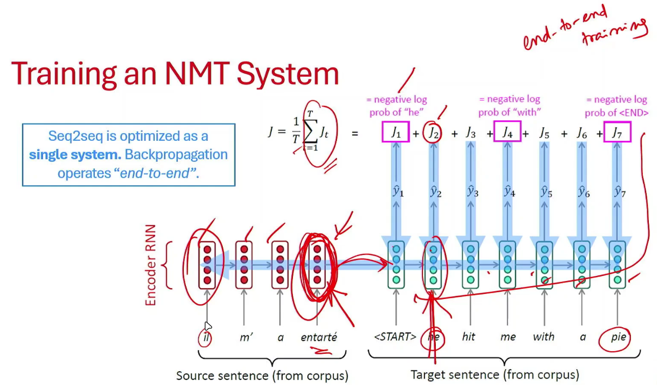
So in an NMT based system we have two blocks : encoder and decoder, so consider an encoder where it takes the embedding of each word from the input sentence one at a time as the input to output an hidden state (vector).

So in short it combines :

• current word embedding $x_t$
• previous hidden state $h_{t-1}$

to produce a new hidden state $h_t$.

That new hidden state serves two purposes:

• Output of the current encoder step
• Memory passed to the next encoder step

Word1 ----> Encoder Cell ----> h1  
|  
v  
Word2 ----> Encoder Cell ----> h2  
|  
v  
Word3 ----> Encoder Cell ----> h3  
|  
v  
...  
|  
v  
WordN ----> Encoder Cell ----> hN


At every step :

h_t = f(x_t, h_{t-1})

After processing the entire sentence, we end up with final hidden state $h_N$ which is the final hidden state. This is the output of the final encoder block in the encoder RNN. The encoder has repeatedly updated this state as it read more words, so ideally $h_N$ contains a compressed representation of the whole sentence.

Now comes the role of decoder, in the original encoder-decoder architecture (before attention, what we are discussing here), the decoder was initialized by this $h_N$ i.e encoder's final hidden state.

The decoder then starts generating the translation one token at a time :

hN
 ↓
"Le"
 ↓
"chat"
 ↓
"s'est"
 ↓
"assis"

The bottleneck becomes obvious :

Source sentence
50 words
      ↓
hN
(single vector)
      ↓
Target sentence
60 words

Everything the decoder needs must pass through that one vector. Other way to look at it is we calculated all those hidden states before calculating $h_N$ why throw them away so that was the insight behind attention.

Instead of :

Decoder ← hN

you get :

Decoder ← {h1, h2, h3, ..., hN}

The decoder can consult whichever encoder states are most relevant while generating each output word. So tldr, bottleneck issue is about final hidden state which doesn't contain all information properly. It contains the information the netowork managed to preserve. In long sentences, a lot of details get diluted or forgotten, all these issues retained in LSTM or GRU which were improvement over vanilla RNNs but attention fixed these issues.

Core Idea behind Attention

On each step of decoder, use a direct connection to the encoder to focus on a particular part of the source sequence, so in a way it helps solve vanishing gradients issue as it is providing a shortcut to faraway states.

Attention ≈ General DL Technique ≈ Given some set of vector values and vector queries, attention is a technique to compute a weighted sum of value, dependent on the query.

Intuition ≈ Weighted Sum ≈ Selective summary of information contained in values, where query determines which value to focus on.

[I know that was very original and definitely 'not bookish language' :)]

So basically we are using a QKV framework, Q ~ Query, K ~ Key and V ~ Value.

• Q : What we are looking for
• K : Labels / Metadata of the items in database (labels of previous states)
• V : Actual information contained in those items

We want to compare the query against all keys to find a match / similarity. Based on similarity / match, retreive the corresponding values.

Let's Consider an example to understand this :

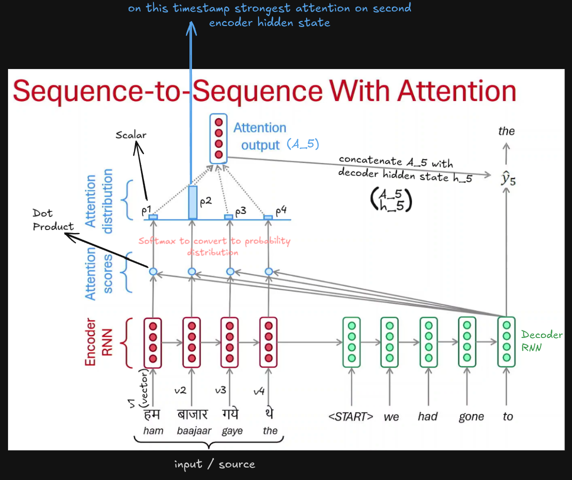
Before starting will be using these things during computation stage :

• score = hᵀe => attention score
• α = softmax(score) => convert to propabilties
• context = Σ αᵢeᵢ => attention / context vector (weighted sum) ~ $A_i$

Suppose we want to translate:

Hindi : हम बाजार गये थे (input)

English : we had gone to the market (output)

Encoder will be reading one word at a time Let's start with first word.

First word: "हम"

Embedding (Assumed) :

x1 = [1,2]

Initial hidden state :

h0 = [0,0]

Encoder combines them :

h1 = [1,1]

Note: How it combines : A simple RNN does : $h_t=tanh⁡(W_x x_t+W_h h_{t−1} + b)$ where, $x_t$ = current word embedding, $h_{t-1}$ = previous hidden state (memory), $W_x, W_h$ = learned weight matrices, $b$ = bias and $tanh$ = activation function

Interpretation :

h1 ≈ information about "हम"

Second word: "बाजार"

Embedding :

x2 = [3,1]

Combine with previous memory :

h2 = [3,2]

Interpretation :

h2 ≈ information about "हम बाजार"

Third word: "गये"

h3 = [2,4] (Assumed)

Contains :

"हम बाजार गये" [h3 will contain info about this phrase in form of an embedding vector]

Fourth word: "थे"

h4 = [1,5]

Contains :

"हम बाजार गये थे"

Encoder outputs :

h1=[1,1]
h2=[3,2]
h3=[2,4]
h4=[1,5]

Old seq2seq (without attention)

Decoder only receives :

h4=[1,5]

Everything must be remembered in this single vector.

Attention version

We keep ALL encoder states :

h1=[1,1]
h2=[3,2]
h3=[2,4]
h4=[1,5]

Now decoder starts generating English.

Decoder timestep 1

We want first output word.

Eventually it should become :

we

Current decoder state :

s1=[2,1]

Think of this as : decoder currently wants the first translated word

Which encoder word is relevant?

Attention asks :

Which encoder hidden state looks most relevant to s1?

We compare :

s1=[2,1]

against every encoder state.

Compare with h1

h1=[1,1]

Dot product :

2×1 + 1×1 = 3

Compare with h2 ([3, 2])

2×3 + 1×2 = 8 (Dot Product)

Compare with h3 ([2, 4])

2×2 + 1×4 = 8 (Dot Product)

Compare with h4 ([1, 5])

2×1 + 1×5 = 7 (Dot Product)

Now we have :

[3,8,8,7] (Attention Score Vector)

These are attention scores. Ones we obtain from blue circles in the above diagram. Now we apply softmax on this to obtain the probability distribution.

[0.003, 0.45, 0.45, 0.097] ≈ [p1, p2, p3, p4] (After applying softmax, sum is 1) 

Interpretation :

0.3% attention on h1
45% attention on h2
45% attention on h3
9.7% attention on h4

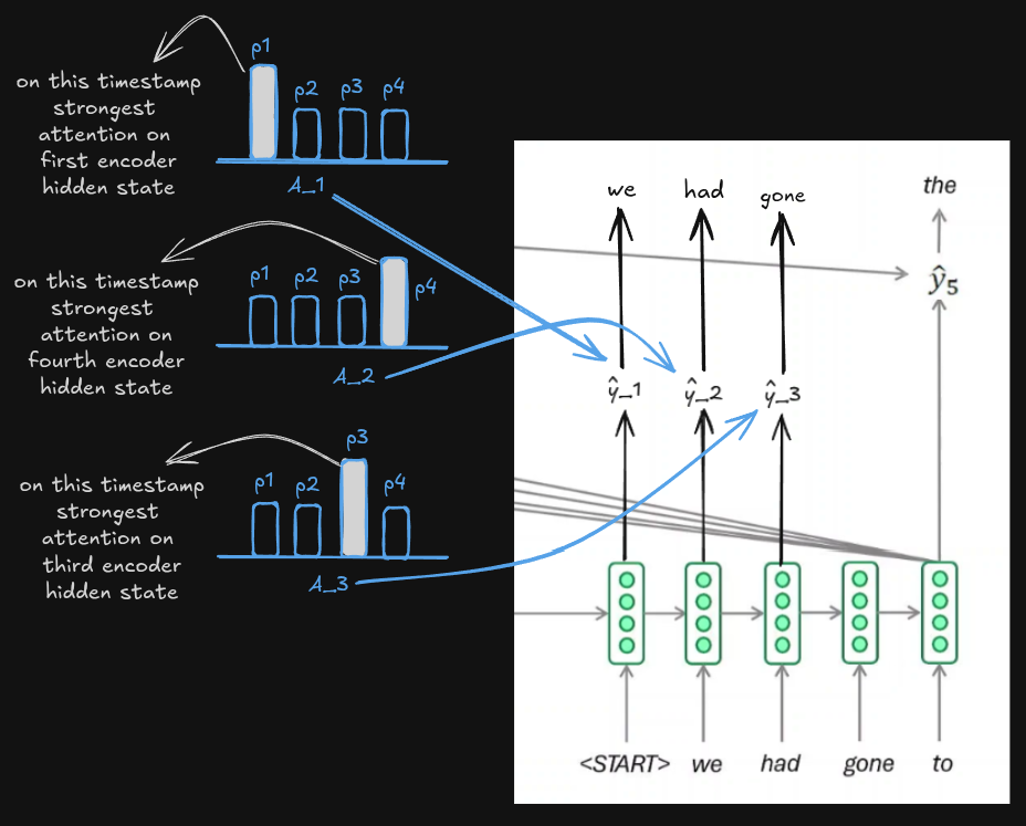
Decoder is mostly looking at encoder positions 2 and 3. The below diagram gives a good idea about the above interpretation

Attention / Context vector

Will build the attention vector now Multiply each encoder state by its weight.

First state :

0.003*[1,1] = [0.003, 0.003]

Second state :

0.45*[3,2] = [1.35,0.90]

Third state :

0.45*[2,4] = [0.90,1.80]

Fourth state :

0.097*[1,5] = [0.097,0.485]

Add everything :

A1 = [2.35, 3.19]

Combine them :

[s1 ; c1] = [2,1, 2.35, 3.19]

Feed into neurnal layer. (Will discuss in detail later in transformer architecture)

Vocabulary probabilities :

we      0.90
had     0.04
gone    0.03
market  0.01

Decoder timestep 2

Now decoder has already generated :

we

Its new hidden state becomes :

s2 = [4,2]

Again compare against all encoder states.

score(s2,h1)
score(s2,h2)
score(s2,h3)
score(s2,h4)

Suppose results :

[2,9,6,1]

Softmax :

[0.001, 0.90, 0.09, 0.009]

Now attention is heavily focused on :

h2

the encoder state corresponding largely to :

बाजार

Create context vector combine with decoder state and predict :

had

Decoder timestep 3

Current sentence :

we had

New decoder state :

s3

Attention scores :

[1,2,10,3]

Softmax :

[0.001, 0.01, 0.97, 0.019]

Now almost all attention is on :

h3

Generate :

gone

Decoder timestep 4

Attention :

[0.01, 0.05, 0.10, 0.84]

Mostly h4.

Generate :

to

Decoder timestep 5

Attention :

[0.01, 0.93, 0.03, 0.03]

Strongly looking back at :

h2

which contains information about :

बाजार

Generate :

market

So that was the core idea behind attention.

Other variants of attention are :

• Original Formulation : $a(q,k) = w_2^T tanh(w_1[q ; k])$
• Bilinear Product : $a(q,k) = q^T Wk$
• Dot Product : $a(q, k) = q^T k$
• Scaled Dot Product : $a(q,k) = \frac{QK^T}{\sqrt{d_k}}$

Single-Head-Self-Attention

So for recap, this is how attention worked : We look at all encoder states, decide which ones matter most right now, take a weighted average of them, and use that information to predict the next word.

At every decoder timestep :

1. Current decoder state asks : Which source positions matter right now?
2. Scores are computed.
3. Softmax converts scores to probabilities.
4. Weighted sum creates context vector.
5. Context + decoder state predicts next word.

And that was attention

Now, what is self-attention ?

For every token :

1. Look at all tokens in the sentence.
2. Decide which ones are important.
3. Gather information from them.
4. Produce a new context-aware representation.

Suppose the sentence is : The animal didn't cross the street because it was too tired.

Question :

What does "it" refer to?

A human immediately knows : it → animal because we can look at other words in the sentence.

A model also needs some way to connect : it ↔ animal even though they are several words apart.

How RNNs tried to solve this

RNNs process sequentially : The → animal → didn't → cross → ... → it For "it" to know about "animal", information must travel through many hidden states :

animal
  ↓
 h2
  ↓
 h3
  ↓
 h4
  ↓
...
  ↓
 h10
  ↓
 it

Long path. Information can weaken or get overwritten.

Self-attention solves this

Instead of passing information step-by-step :

animal
  ↓
 h3
  ↓
 h4
  ↓
...
  ↓
 it

the token "it" can directly look at every token :

     it
 ↙    ↓   ↘
The animal didn't cross ...

and decide :

animal : 85%
street : 5%
cross  : 3%
other  : 7%

Then it gathers information mostly from animal. That's self-attention.

Without self-attention :

Token representation = information about itself

With self-attention :

Token representation = information about itself + information from relevant tokens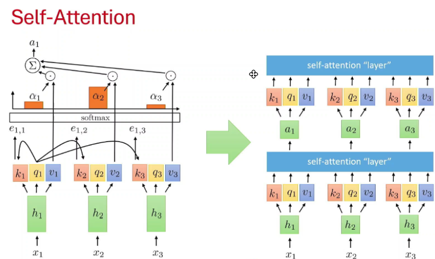

Consider the sentence as an example :

I love pizza

After embeddings :

x1 = "I"
x2 = "love"
x3 = "pizza"

Each token is projected into :

Query (Q)
Key   (K)
Value (V)

So :

Token 1 ("I") : q1, k1, v1
Token 2 ("love") : q2, k2, v2
Token 3 ("pizza") : q3, k3, v3

What are we trying to compute?

We want a new representation for token 1.

The model asks:

While processing "I", how much should I pay attention to:

• myself ("I")?
• "love"?
• "pizza"?

Step 1: Compare q₁ against every key

Compute :

e₁₁ = q₁ · k₁
e₁₂ = q₁ · k₂
e₁₃ = q₁ · k₃

Suppose :

e₁₁ = 2
e₁₂ = 8
e₁₃ = 4

Meaning :

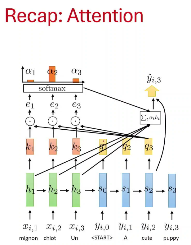
"I" is most related to "love"

according to the learned representations. These are the black arrows in figure.

Step 2: Softmax

Convert scores into probabilities :

[2, 8, 4]

   ↓

  softmax

   ↓

α₁ = [0.002, 0.98, 0.018]

These are the orange bars.

Interpretation :

0.2% attention on token 1
98% attention on token 2
1.8% attention on token 3

So token 1 is looking mostly at token 2.

Step 3: Weighted sum of values

Now use those attention weights on the values :

a₁ =0.002*v₁ + 0.98*v₂ + 0.018*v₃

This produces :

a₁

which is the output vector at the top left of above diagram.

What does a₁ mean?

Originally token 1 only knew :

"I"

After self-attention :

a₁

contains information from :

"I"+"love"+"pizza"

mostly from "love". So token 1 now has context from the entire sentence.

Then do the same for token 2

Now process :

q₂

against all keys :

q₂·k₁
q₂·k₂
q₂·k₃

Suppose :

[5,2,9]

Softmax :

[0.1, 0.02, 0.88]

Then :

a₂ = 0.1*v₁ + 0.02*v₂ + 0.88*v₃

Token 2 now mostly gathers information from token 3.

Then token 3

Same thing :

a₃ = α₃₁v₁ + α₃₂v₂ + α₃₃v₃

Why is it called SELF-attention?

Because :

q₁,q₂,q₃
k₁,k₂,k₃
v₁,v₂,v₃

all come from the same sentence.

The tokens are attending to each other.

I      ↔ love
love   ↔ pizza
pizza  ↔ I

No encoder-decoder interaction.

The one-sentence summary of self-attention is :

For each token, compare its query with every token's key to determine importance, use softmax to get attention weights, then take a weighted average of the value vectors to create a context-aware representation of that token.

Multi-Head-Self-Attention

Instead of calculating attention once, MHA repeats the QKV process multiple times simultaneously. Each repetition uses completely different, independent set of learnable weight matrices ($W_Q, W_K. W_V$). Each separate set is "attention head".

It is similar to CNNs, where different kernels capture different patterns / features of an image. MHA takes inspiration from this, the way a image has many visual features, a word in a sentence has different linguistic and semantic relation, using MHA, the transformer can fetch different types of information from same token simultaneously.

Consider an example,

Head 1 --> act as a grammer checker, focus on identifying if word is subject or verb Head 2 --> act as a vocabulary checker, checking if the word is noun, pronoun or named entity Head 3 --> look for context, map a pronoun like "it" back to noun it refers to

Head 1 : WQ₁ WK₁ WV₁
Head 2 : WQ₂ WK₂ WV₂
Head 3 : WQ₃ WK₃ WV₃ 

Each head learns different behavior. All heads are looking at same sentence - same tokens but each head develops a different specialization

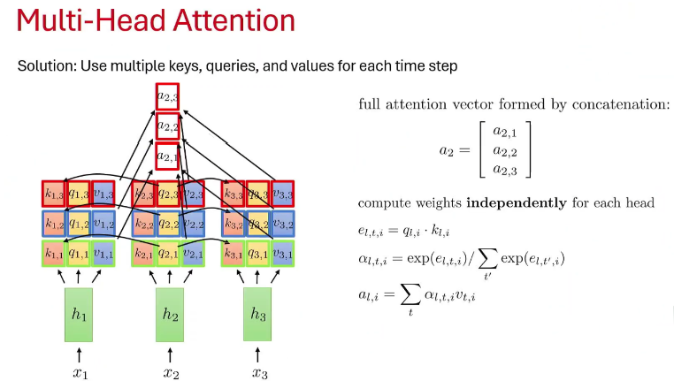
($q_{~ time-step,~ head-number}$ ) is the notation used in above diagram. All heads operate in parallel, $q_{~ 2, ~ 1}$ , $q_{~ 2, ~ 2}$ , $q_{~ 2, ~ 3}$ all calculate attention score simultaneously.

Self-attention :

One expert reads the sentence and tells each token what is important.

Multi-head attention :

Eight different experts read the same sentence. Each expert notices different relationships. Their observations are combined into a richer representation. Instead of one perspective there are multiple perspective now.

MHA is just multiple independent self-attention mechanisms running in parallel on the same sequence, each with its own learned view of the sentence.

Consider the example :

I love pizza

We'll use 2 attention heads

Step 0: Input embeddings

Suppose embeddings are :

I = [1,0]
love = [2,1]
pizza = [0,2]

Let's focus on token :

love

because that's where we'll compute attention.

SINGLE HEAD ATTENTION

Assume for simplicity :

Q = K = V = embedding

(Not true in real transformers, but easier to understand.)

So :

q_love = [2,1]

Compare against every token

love with I

[2,1]·[1,0]= 2

love with love

[2,1]·[2,1]= 5

love with pizza

[2,1]·[0,2]= 2

Scores :

[2,5,2]

Apply Softmax

Approximately :

[0.045, 0.91, 0.045]

Interpretation :

4.5% attention on I
91% attention on love
4.5% attention on pizza

Weighted sum

Values :

v1=[1,0]
v2=[2,1]
v3=[0,2]

Compute :

0.045*v1 + 0.91*v2 + 0.045*v3

Result :

a = [1.87, 1.00]

This is the output of the attention layer.

Problem

Only one attention pattern exists :

[0.045,0.91,0.045]

One view of the sentence. Maybe that's enough or maybe not.

MULTI-HEAD ATTENTION

Now create TWO heads. Each head gets different learnable matrices.

HEAD 1

Suppose Head 1 learns :

"Focus on grammatical structure"

Its projections become :

q_love^(1)=[1,1]

Keys :

$k_{I}^1=[1,1]$ $k_{love}^1=[1,2]$ $k_{pizza}^1=[0,1]$

Scores

love vs I = 1×1 + 1×1 = 2

love vs love = 1×1 + 1×2 = 3

love vs pizza= 1×0 + 1×1 = 1

Scores :

[2,3,1]

Softmax :

[0.24, 0.66, 0.10]

Head 1 mostly focuses on :

love

Head 1 output

Values :

$v_I^1 = [1,0]$ $v_{love}^1 = [2,1]$ $v_{pizza}^1 = [0,1]$

Weighted sum :

0.24*[1,0] + 0.66*[2,1] + 0.10*[0,1] = a1 = [1.56,0.76]

HEAD 2

Suppose Head 2 learns :

"Look for semantic objects"

Different matrices produce : $q_{love}^2=[1,3]$

Keys : $k_I^2=[0,1]$ $k_{love}^2=[1,1]$ $k_{pizza}^2=[1,3]$

Scores

I :

[1,3]·[0,1] = 3

love :

[1,3]·[1,1] = 4

pizza :

[1,3]·[1,3] = 10

Scores :

[3,4,10]

Softmax :

[0.001, 0.002, 0.997]

Head 2 is screaming :

LOOK AT PIZZA

which is reasonable. "love" is usually about something.

Head 2 output

Values:

v_I^2 = [1,1]
v_{love}^2 = [2,0]
v_{pizza}^2 = [5,5]

Weighted sum ≈ [4.99,4.99] So, a2=[4.99,4.99]

Combine heads

Head outputs :

a1=[1.56,0.76] 
a2=[4.99,4.99]

Concatenate :

[a1 ; a2] = [1.56, 0.76, 4.99, 4.99]

This becomes the representation of :

love

after Multi-Head Attention.

Why is this better ?

Single head produced :

[1.87,1.00]

based on ONE attention pattern.

Multi-head produced :

Head 1 : grammar-ish information
Head 2 : object/semantic information

combined into one richer vector.

What each head "sees"

For the same token "love":

Head 1 :

I      24%
love   66%
pizza  10%

Head 2 :

I      0.1%
love   0.2%
pizza  99.7%

Notice :

• same sentence
• same token
• completely different attention patterns

That's the entire reason Multi-Head Attention exists.

A single head asks:

"What is important?"

Multiple heads ask:

"What is important from several different perspectives simultaneously?"

Summary

In Self-Attention, Q, K, V all come from same sequence, every word in sentence is simultaneously acting as searcher, target and actual information being shared.

"The animal didn't cross the street as it was too tired"

We know "it" refers to animal but not the computer, it only sees isolated tokens. Each word here is multiplied by 3 separate matrices ($W_K, W_Q, W_V$) to generate its own Q, K, V.

"it" => $Q_{it}, K_{it}, V_{it}$ and "street" => $Q_{street}, K_{street}, V_{street}$ etc... (single set of 3 matrices exist for each word)

and to figure out the relation / context take the dot product (compare) against key of every other word in sentence.

$K_{street}$ => singular noun but inanimate (low match) => can apply softmax to get probabilities

$K_{animal}$ => singular noun but animate (high match) => can apply softmax to get probabilities

$Q_{it}$ => needs a single noun (which is capable of being tired) & its a pronoun

This means "animal" gets 80% attention, "street" gets 5% attention, other words share the remaining 15%

"it" knows who it should pay attention to collects value(V) of all words => 80% of $V_{animal}$ , 5% of $V_{street}$ , etc and adds them for attention vector => model figured out how words relate to other ("it" is looking at its own sentence to find answers)

How it compares to MHA ?

In SHA, only one head was there so it needed to balance all rules of english at once, which was a messed up mixture lacking nuance, in MHA, we can look at the sentence from multiple perspective (each perspective = separate head = separate QKV set) where each perspective can ask specific query then concatenation is done.