Positional Encoding 101

Why Need Positional Encoding ?

So unlike older sequential models, transformers process all tokens simultaneously in parallel which makes training efficient but creates a blind spot : the self-attention mechanism is simply a set of linear operations and dot products which have no concept of sequence order. Without any kind of intervention, the model wouldn't know the difference between "The dog chased the pig" and "The pig chased the dog"

So how can we fix this ?

• We can inject position into the inputs. To give the model a sense of order, we can create a distinct "position vector" which is the exact same dimension as the semantic word embedding. These two vectors are summed together .

• Why sum instead of concatenate ? While concatenation is mathematically possible, summing them keeps the vector size constant, which heavily reduces the parameter count and memory footprint in subsequent layers.

• The positional vector is added only at the very beginning of the network (before the first encoder or decoder block). It is not continuously re-added at every deep layer.

Some failed attempts at positional encoding :

1. The Simple Counting Method (Option 1)

• The Idea: The most intuitive way to track position is to just assign position 0 a vector of all zeros, position 1 a vector of all ones ([1,1,1,1]), and position 30 a vector of all thirties ([30,30,30,30]).

• The Flaw: Sentence lengths vary wildly, and the numbers grow unbounded. If a sequence only has three words, the final embedding is [3,3,3,3]. If a sequence has 30 words, the final embedding is [30,30,30,30]. The model might misinterpret a [3,3,3,3] vector, not knowing if it represents the absolute end of a short sentence or just the beginning of a long one.

2. The Normalized Counting Method (Option 2)

• The Idea: To fix the unbounded growth problem, you could divide the position number by the maximum length of the sequence. This guarantees that the final word in any sentence is always encoded as [1,1,1,1], regardless of how long the sentence is.

• The Flaw: This makes the positional embedding dependent on the sequence length. As in a 4-word sentence (N=4), the embedding for position 1 is [0.33, 0.33, 0.33, 0.33]. But in a 5-word sentence (N=5), the embedding for position 1 changes to [0.20, 0.20, 0.20, 0.20]. This is a failure because we need a consistent, unique vector for "Position 1" every time, no matter how long the surrounding sentence is.

3. The Binary Breakthrough

• The Idea: To get consistent vectors that don't grow infinitely large, the instructor looks at how binary counting works (000, 001, 010, 011, etc.).

• The Insight: If you look closely at the columns in that binary image, a pattern emerges. The rightmost column (least significant bit) alternates rapidly: 0, 1, 0, 1. The next column to the left alternates slower: 0, 0, 1, 1. The next column is even slower: 0, 0, 0, 0, 1, 1, 1, 1.

• The Conclusion: Binary counting reveals a predictable, repeating pattern of varying frequencies. Simply adding rigid binary 0s and 1s to the fractional numbers of continuous word embeddings doesn't work well mathematically. However, this concept of using varying frequencies is the exact inspiration for the final Transformer solution: using smooth, continuous sine and cosine waves of different frequencies to encode position instead of discrete binary bits.

Maths behind Positional Encoding

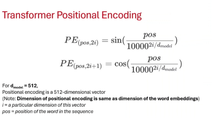
Every element in the positional vector is generated using either a sine or a cosine function :

• Even dimensions ($2i$): Use the sin function.

• Odd dimensions ($2i+1$): Use the cos function.

• The Variables :

  • pos: The absolute position of the word in the sequence (0, 1, 2, etc.).

  • i: The dimension index within the vector (0, 1, 2... up to $d_{model}/2$).

  • d_model: The total size of the embedding vector (e.g., 512).

The crucial part of this formula is the denominator: $10000^{2i / d_{model}}$. As the dimension index $i$ increases, this denominator gets exponentially larger. This means that early dimensions in the vector (where $i$ is small) have high frequencies, while later dimensions (where $i$ is large) have very low frequencies.

More on '$i$' and '$d_{model}$'

Word embedding is a vector of size 512 (so, $d_{model} = 512$). (Basically if I'm converting a word to its embedding it's vector size will be 512) The positional encoding must also be a vector of size 512 so they can be added together.

The formula uses sine for even positions in the vector and cosine for odd positions. Therefore, they are generated in pairs. The variable $i$ simply represents the index of the pair.

Since we have 512 total dimensions, we have 256 pairs. Therefore, $i$ counts from 0 to 255.

• For pair $i=0$: Dimension 0 uses sine, Dimension 1 uses cosine.
• For pair $i=1$: Dimension 2 uses sine, Dimension 3 uses cosine.
• ...
• For pair $i=255$: Dimension 510 uses sine, Dimension 511 uses cosine.

The denominator formula is: $10000^{2i / d_{model}}$

This denominator is an important term here. Its entire job is to grow exponentially larger as you move deeper into the vector (as $i$ increases). Let's calculate the denominator at three different points in our 512-dimensional vector to see what happens to a word at Position 1 ($pos = 1$).

Example A: The Very First Dimensions ($i = 0$)

Let's look at the first pair of dimensions (Dimensions 0 and 1).

• The Exponent: $2(0) / 512 = 0$

• The Denominator: $10000^0 = 1$

• The Math: $\sin(pos / 1)$ $\rightarrow$ $\sin(1 / 1)$ $\rightarrow$ $\sin(1)$

Because the denominator is just 1, the sine wave is unmodified. It fluctuates very rapidly. If you move from word position 1 to word position 2, the output changes drastically.

Example B: The Middle Dimensions ($i = 128$)

Let's look exactly halfway through our vector (Dimensions 256 and 257).

• The Exponent: $2(128) / 512 = 256 / 512 = 0.5$

• The Denominator: $10000^{0.5}$ (which is the square root of 10000) = 100

• The Math: $\sin(pos / 100)$ $\rightarrow$ $\sin(1 / 100)$ $\rightarrow$ $\sin(0.01)$

Now we are dividing the position by 100 before taking the sine. This stretches the wave out by a factor of 100. It takes 100 words for this specific dimension to complete the same cycle that the first dimension completed in just one word !

Example C: The Very Last Dimensions ($i = 255$)

Let's look at the very end of our vector (Dimensions 510 and 511).

• The Exponent: $2(255) / 512 = 510 / 512 \approx 1$

• The Denominator: $10000^1 = 10000$

• The Math: $\sin(pos / 10000)$ $\rightarrow$ $\sin(1 / 10000)$ $\rightarrow$ $\sin(0.0001)$

The denominator is now massive. This wave is stretched out so far that over the course of a normal sentence, this value barely changes at all. It acts almost like a constant, gentle slope.

Simple Dry-Run :

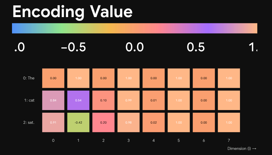
Imagine we have a tiny Transformer where the word vectors are only 4 dimensions long ($d_{model} = 4$). We want to encode the positions for a simple 3-word sentence: "The cat sat."

Because our vector only has 4 slots, we only have two pairs to calculate:

• Pair 1 ($i = 0$): Fills Dimensions 0 and 1.
• Pair 2 ($i = 1$): Fills Dimensions 2 and 3.

Let's calculate the denominators for our two pairs :

• For $i = 0$: The denominator is $10000^{2(0)/4} = 10000^0 = \mathbf{1}$.
• For $i = 1$: The denominator is $10000^{2(1)/4} = 10000^{0.5} = \mathbf{100}$.

Now, let's watch what happens to the math as we move word by word.

Step-by-Step for "The cat sat"

Word 1: "The" ($pos = 0$)

• Dim 0 ($i=0, \sin$): $\sin(0 / 1) = \mathbf{0.00}$

• Dim 1 ($i=0, \cos$): $\cos(0 / 1) = \mathbf{1.00}$

• Dim 2 ($i=1, \sin$): $\sin(0 / 100) = \mathbf{0.00}$

• Dim 3 ($i=1, \cos$): $\cos(0 / 100) = \mathbf{1.00}$

• Final Position Vector for "The": [0.00, 1.00, 0.00, 1.00]

Word 2: "cat" ($pos = 1$)

• Dim 0 ($i=0, \sin$): $\sin(1 / 1) = \mathbf{0.84}$

• Dim 1 ($i=0, \cos$): $\cos(1 / 1) = \mathbf{0.54}$

• Dim 2 ($i=1, \sin$): $\sin(1 / 100) = \sin(0.01) = \mathbf{0.01}$

• Dim 3 ($i=1, \cos$): $\cos(1 / 100) = \cos(0.01) = \mathbf{0.99}$

• Final Position Vector for "cat": [0.84, 0.54, 0.01, 0.99]

Word 3: "sat" ($pos = 2$)

• Dim 0 ($i=0, \sin$): $\sin(2 / 1) = \mathbf{0.91}$

• Dim 1 ($i=0, \cos$): $\cos(2 / 1) = \mathbf{-0.42}$

• Dim 2 ($i=1, \sin$): $\sin(2 / 100) = \sin(0.02) = \mathbf{0.02}$

• Dim 3 ($i=1, \cos$): $\cos(2 / 100) = \cos(0.02) = \mathbf{0.99}$

• Final Position Vector for "sat": [0.91, -0.42, 0.02, 0.99]

Look closely at the resulting vectors : s

1. The "Fast" Dimensions (0 & 1): From word 0 to word 2, the sine value jumped wildly from 0.00 to 0.84 to 0.91. The cosine value dropped from 1.00 to 0.54 to -0.42. Because the denominator was small ($1$), these numbers change drastically with every single step. This is how the model tells two side-by-side words apart.

2. The "Slow" Dimensions (2 & 3): From word 0 to word 2, the sine value barely crept up from 0.00 to 0.01 to 0.02. Because the denominator was large ($100$), these numbers are barely moving. If this sentence were 500 words long, these slow dimensions would smoothly curve over the length of the whole paragraph, letting the model know if a word is at the beginning, middle, or end of a document.

Differentiating between Nearby and Distant Words

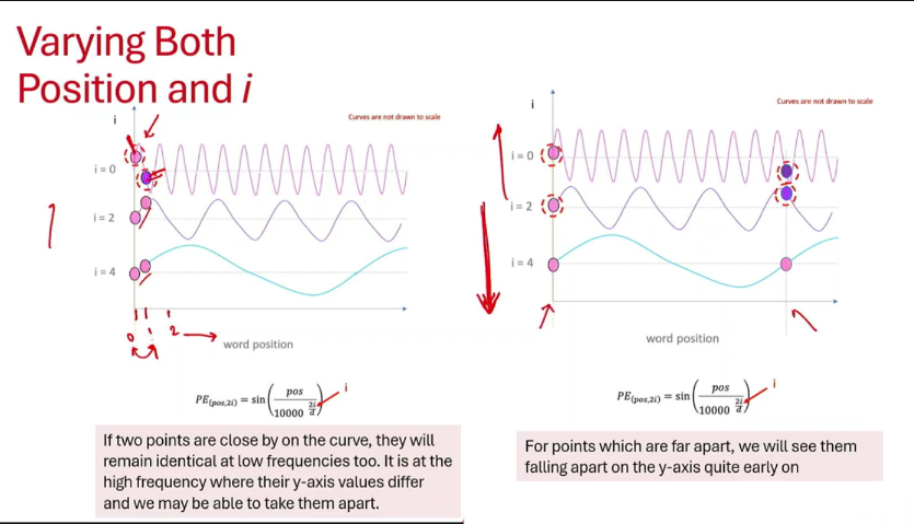
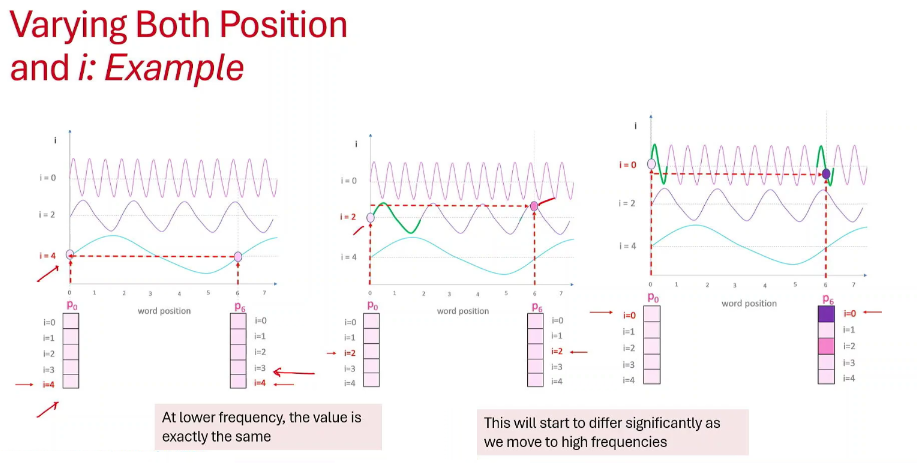
Transformer uses a mix of different wave frequencies to help differentiate between nearby and distant words, model figures out where a word is located using only the height of a wave (the y-value). We use High Frequency waves and Low Frequency waves for this purpose Here is why we need both extremes to make the system work.

1. The High-Frequency Waves (The "Fast" Waves)

These are the sine waves generated in the first few dimensions of the positional encoding vector. They cycle up and down very quickly.

• What they do well (Nearby Words): Because they move so fast, the wave's height changes dramatically from one word to the very next. For example, at pos=0, the wave might be at its peak (1.0). By pos=1, it has already crashed down to its valley (−1.0). This massive difference makes it incredibly easy for the model to tell that these two words are right next to each other but in different spots.

• Where they fail (Distant Words): The problem with a fast wave is that it repeats itself constantly. By the time you get to pos=6, the wave might have cycled completely and hit the peak (1.0) again. If the model only had this fast wave, it would look at the height of 1.0 and be unable to tell if the word was at position 0, 2, 4, or 6.

2. The Low-Frequency Waves (The "Slow" Waves)

These are the waves generated in the later dimensions of the vector. They are stretched out so massively that it might take hundreds of words just to complete a single up-and-down cycle.

• What they do well (Distant Words): Because the cycle takes so long, a word at pos=0 and a word at pos=50 will have vastly different heights on this wave. Word 0 might be at 0.0, while word 50 might be at 1.0. The model can easily use this wave to tell that these words are far apart.

• Where they fail (Nearby Words): Because the wave is so stretched out, the slope is incredibly flat. The height of the wave at pos=0 might be 0.000, and the height at pos=1 might be 0.001. To a neural network, those numbers are nearly identical. If it only relied on this slow wave, it would blur nearby words together, unable to distinguish "The cat" from "cat The".

If the model only looks at the fast waves, it gets confused by distant words. If it only looks at the slow waves, it gets confused by nearby words. By stacking 512 of these waves together, ranging from lightning-fast to incredibly slow, every single word position in a sentence gets a completely unique fingerprint. When the model needs to distinguish between word 1 and word 2, it relies heavily on the first few numbers in the vector (the fast waves - high frequency). When it needs to know if a word is at the beginning of a paragraph or the end of a paragraph, it relies heavily on the last few numbers in the vector (the slow waves - low frequency).

The Left Graph: The Problem with Nearby Words

Look at the two red dotted lines clustered tightly together on the left side (representing two words right next to each other, like Position 0 and Position 1).

1. Follow the lines down to the bottom blue wave: Look at the two pink dots on the blue line. They are at almost the exact same height. The wave is so flat here that the values are nearly identical. If the network only looked at this blue wave, it would suffer from "order blur" and mix the words up.
2. Follow the lines up to the top purple wave: Look at the dots circled in red. One dot is at the peak, and the other is lower down. They have vastly different vertical heights.

What it conveys: We need high-frequency waves to tell adjacent words apart, because low-frequency waves are too flat.

The Right Graph: The Problem with Distant Words

Now look at the right graph. The red dotted lines are now far apart (representing Word 0 and Word 6).

1. Follow the lines up to the top purple wave: Look at the two dots circled in red. Because the purple wave cycles up and down so rapidly, the dot at Position 0 and the dot at Position 6 happen to land at the exact same vertical height. If the network only looked at this purple wave, it would think Word 0 and Word 6 were sitting in the exact same chair! It has no idea how far apart they are because the pattern repeats too fast.
2. Follow the lines down to the bottom blue wave: Look at the pink dots on the blue line. One is at the middle baseline, and the other is way up near the peak.

What it conveys: We need low-frequency waves to measure long distances, because high-frequency waves repeat themselves and cause distant words to accidentally overlap.

Think of the phrase: "Dog bites man."

• "Dog" is at Position 0.
• "bites" is at Position 1.
• "man" is at Position 2.

"Dog" and "bites" are next to each other. But if the model mixes up their different spots, the sentence becomes "Man bites dog", which means something entirely different. The model / neural network needs a mathematical way to look at "Dog" and "bites" and understand these words are next to each other but are at different positions.

Neural network doesn't understand English; it only reads numbers. To a neural network, numbers that are close together look "similar."

• If Word 0 gets the position number 0.001
• And Word 1 gets the position number 0.002

To the network, these numbers are nearly identical. It might struggle to tell which one came first, blurring the strict order of the sentence. We need a math function that takes one tiny horizontal step forward (from Word 0 to Word 1) but results in a massive vertical jump.

This is the actual math for that first dimension wave ($\sin(pos / 1)$) :

• Position 0: $\sin(0)$ = 0.00
• Position 1: $\sin(1)$ = 0.84

That jump from 0.00 to 0.84 is massive in the world of neural networks (where numbers generally live between -1.0 and 1.0). Because the value changed so rapidly, the model looks at Word 0 and Word 1 and understands their values differ significantly and must not mess up their position.

Postional Encoding vs Word Embedding

The positional encoding only carries information about time/location. It is completely blind to semantics. To see why a small difference in the wave causes a catastrophic failure, we have to look at the two different vectors that are being added together before the network even starts processing:

1. The Word Embedding (The "Meaning")

Before a word ever sees a sine wave, it gets converted into a Word Embedding. This is where the actual meaning lives.

• In this space, "cat" and "dog" have very similar numbers because they are both pets.
• "Cat" and "carburetor" have wildly different numbers.
• This vector says: "I am a furry animal that meows."

2. The Positional Encoding (The "Seat Number")

This is our sine wave vector. It knows nothing about cats or dogs.

• This vector simply says: "I am sitting in Chair #1."

The Transformer takes the Meaning Vector and adds it to the Positional Vector. The final result is a combined vector that essentially says: "I am a furry animal that meows, and I am sitting in Chair #1."

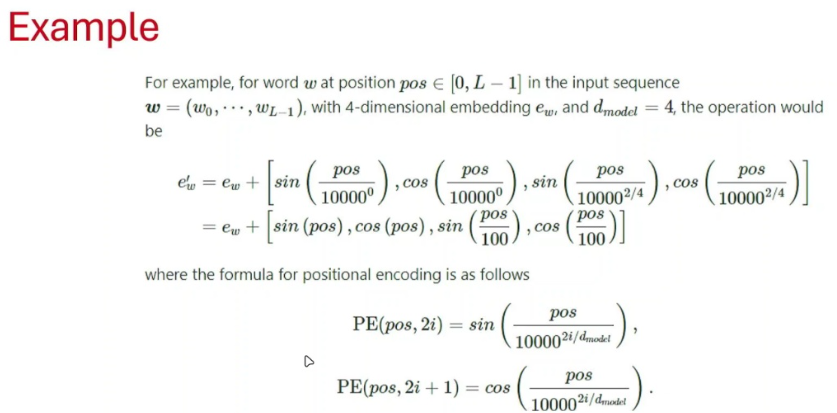
Equation used : $e'_w = e_w + [ \text{Positional Encoding Vector} ]$

• $w$: The specific word we are looking at (like "cat").
• $pos$: The absolute index of that word in the sentence (0, 1, 2, etc.).
• $e_w$: The Word Embedding vector. This is the array of 4 numbers that holds the meaning of the word.
• $e'_w$: The final combined vector (Meaning + Position) that gets fed into the Transformer.

Think of the Positional Encoding like printing seat numbers on movie tickets:

• High-Frequency Wave (Clear Printing): Word 0 gets ticket #0.00. Word 1 gets ticket #0.84. The neural network (the usher) looks at the tickets, sees a massive difference, and perfectly seats "Dog" in Chair 0 and "bites" in Chair 1. Order is maintained.

• Low-Frequency Wave (Smudged Printing): Word 0 gets ticket #0.001. Word 1 gets ticket #0.002. To a neural network, these numbers are basically identical. The usher gets confused. It looks at "Dog" and "bites" and says, "Your tickets look exactly the same. I don't know who goes first."

If the model relies only on those slow waves for words that are right next to each other, it suffers from order blur. It knows the words "Dog", "man", and "bites" are in the sentence (because of the word embeddings), but it has lost the seat numbers. It might accidentally read "Dog bites man" as "Man bites dog." The words didn't change meaning; the network just literally forgot what order they were standing in.

Rules any Positional Encoding Method must follow

Any positional encoding method, should ideally obey three mathematical properties, evaluated by a proximity function $\phi~(x, y)$:

• Monotonicity: If two words are pushed further apart, their positional proximity score must decrease.
• Translation Invariance: The relative relationship between two words shouldn't change just because you shifted the whole sentence. "The dog chased the pig" and "Yesterday, the dog chased the pig" should preserve the exact same positional relationship between "dog" and "pig".
• Symmetry: The distance from Word A to Word B should be the same as the distance from Word B to Word A.

Relative Positions

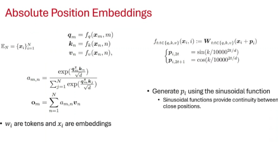
Absolute Positional Encoding (The Original Method) : Think of this like assigning strict GPS coordinates or exact positton to every word in a sentence.

• Word 0 gets the vector for "Position 0".
• Word 5 gets the vector for "Position 5".

This is what the sine/cosine waves (or learned absolute vectors) do. They are added to the word before the neural network does any processing.

• The Flaw: Language doesn't care about absolute positions. If I say "The dog chased the cat" or "Yesterday, the dog chased the cat," the relationship between "dog" and "cat" is identical. But under Absolute Encoding, their positions completely changed. The neural network has to expend massive computational effort relearning how "Position 1 to Position 4" relates to "Position 2 to Position 5." Furthermore, it struggles if you ask it to process a 2000-word document when it was only trained on 1000-word documents, because it has never seen those other position relations.

Relative Positional Encoding (The Modern Method)

Think of this like giving directions: "Take three steps to the right." Instead of assigning a position, the network only looks at the distance between two words when they are paying attention to each other.

• The Advantage: If "dog" is querying "cat", the relative distance is $+3$. It does not matter if this happens at the beginning, middle, or end of a book; the distance is always $+3$. This is called Translation Invariance, and it allows models to generalize beautifully to longer texts.

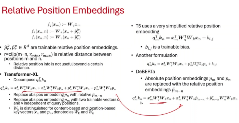
If Relative Encoding is so much better, why didn't Vaswani use it in the original 2017 paper? Because mathematically, it is very difficult to inject distances into the standard Transformer architecture. Let's have to look at what happens when a Query ($q$) at position $m$ pays attention to a Key ($k$) at position $n$. If you take the standard Absolute method ($Word + Position$) and multiply them together ($q_m^T k_n$), algebra dictates that it expands into four distinct terms :

1. Word to Word: ($x_m^T W_q^T W_k x_n$) $\rightarrow$ Does the meaning of Word A care about the meaning of Word B ?

2. Word to Position: ($x_m^T W_q^T W_k p_n$) $\rightarrow$ Does the meaning of Word A care about the absolute location of Word B ?

3. Position to Word: ($p_m^T W_q^T W_k x_n$) $\rightarrow$ Does the absolute location of Word A care about the meaning of Word B ?

4. Position to Position: ($p_m^T W_q^T W_k p_n$) $\rightarrow$ Does the absolute location of Word A care about the absolute location of Word B ?

1. Transformer-XL (The Surgical Hack)

The Transformer-XL team looked at those four expanded terms and decided to manually rewrite them:

• They completely removed the absolute key position ($p_n$) in terms 2 and 4, replacing it with a relative distance vector ($p_{m-n}$).
• For the query's absolute position ($p_m$) in terms 3 and 4, they realized that since the query is the "reference point" looking out at the rest of the sentence, its absolute position doesn't matter. They replaced it with simple, trainable bias vectors ($u$ and $v$).
• The Result: The model no longer calculates attention based on where words are absolutely located, but rather on how far apart they are.

2. DeBERTa (Disentangled Attention)

DeBERTa took a very similar approach to Transformer-XL but made it cleaner. Instead of completely separating the position from the word early on, they explicitly replaced the absolute embeddings ($p_m$ and $p_n$) inside the expanded dot-product with relative position embeddings ($\tilde{p}_{m-n}$). They called this "disentangled attention" because it computes the content-to-content (word meaning) and position-to-position (distance) scores separately before adding them together.

3. T5 (The Elegant Simplification)

The researchers behind the T5 (Text-to-Text Transfer Transformer) model looked at this massive, complicated algebra and decided to throw it in the trash.

• They removed positional vectors from the input entirely.
• They calculated the attention score using only the meanings of the words ($x_m^T W_q^T W_k x_n$).
• Then, right at the very end, they simply added a single learned number (a scalar bias, $b_{i,j}$) to the final score based purely on the distance between the two words.
• The Result: If Word A is 3 steps away from Word B, the model just looks up the learned bias value for "+3 steps" and adds it to the attention score. It is incredibly simple, highly effective, and entirely relative.

Rotatory Positional Encoding (RoPE)

This is the modern way for positional encoding. Previous methods added a position vector to the word embedding. RoPE, instead, multiplies the word embedding by a rotation matrix.

Imagine a word embedding as a 2D vector (an arrow pointing in a specific direction).

• The length of the arrow represents the word's meaning.
• To encode its position (e.g., Position 3), RoPE simply rotates that arrow by a specific angle.

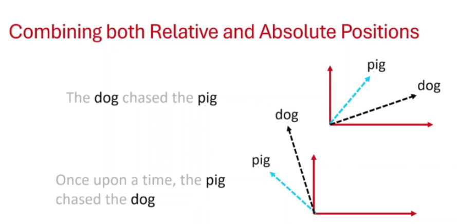
If "dog" is at Position 0 and "pig" is at Position 3, there is a specific angle between their two arrows. If you shift the sentence so "dog" is at Position 5 and "pig" is at Position 8, both arrows get rotated further by the same amount. Therefore, the relative angle between them remains exactly the same. Since the attention score ($Q^T K$) is essentially measuring the angle (dot product) between two vectors, the model naturally preserves relative distance while explicitly calculating absolute positions.

Maths behind RoPE

I won't go into the very depth of the maths behind this as it can be a separate article in itself. So main logic is using complex numbers to force absolute positions to subtract themselves during the attention calculation.

Before RoPE, positional encoding was purely real-number vector addition. The RoPE authors realized that if they mapped word embeddings into the complex plane (where numbers have a real part and an imaginary part, like $x + iy$), they could unlock a specific mathematical tool: Euler's Formula ($e^{i m \theta} = \cos(m\theta) + i\sin(m\theta)$).

Euler's formula states that multiplying a number by $e^{i\theta}$ simply rotates it around a circle by angle $\theta$.

• Let's say we have a word embedding vector for a Query ($q$) and a Key ($k$). We chop them into 2D pairs.
• We assign a base rotation angle, $\theta$.
• To encode that the Query is at absolute position $m$, we multiply it by $e^{im\theta}$. This rotates the Query vector by $m$ steps.
• To encode that the Key is at absolute position $n$, we multiply it by $e^{in\theta}$. This rotates the Key vector by $n$ steps.

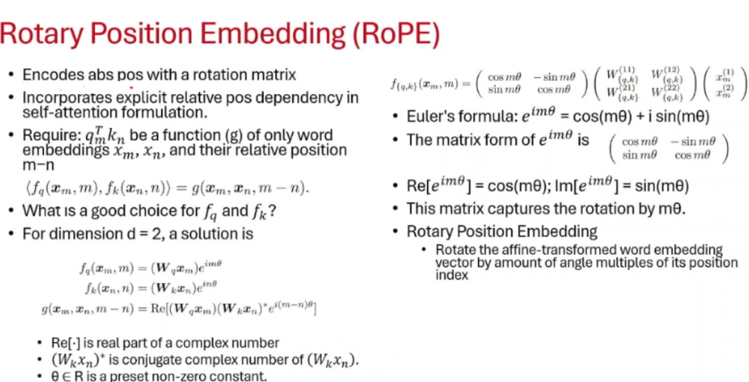
The self-attention mechanism calculates the dot product between the Query and the Key. In the world of complex numbers, calculating a dot product requires taking the complex conjugate of the second vector.

Taking the complex conjugate simply flips the sign of the imaginary exponent. So, the Key's rotation $e^{in\theta}$ becomes $e^{-in\theta}$.

Now, this is what happens to the exponents when the attention mechanism multiplies the Query and the Key together:

$(q \cdot e^{im\theta}) \times (k \cdot e^{-in\theta})$

Because of the rules of exponents, the math naturally combines them:

$(q \cdot k) \times e^{i(m-n)\theta}$

Look at the exponent: $(m-n)$.

The absolute position of the Query ($m$) and the absolute position of the Key ($n$) have completely vanished. The math naturally subtracted them, leaving only their relative distance. The network explicitly encoded absolute positions, but the attention mechanism mathematically only sees the distance between them.

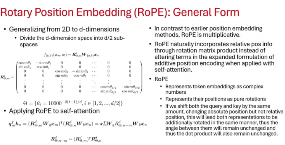
The math above works perfectly if word embeddings are only 2 dimensions long. But in modern models, embeddings are massive, often 4096 dimensions or more. You cannot rotate a 4096-dimensional vector using a simple 2D complex plane trick.

To solve this, the authors generalize the math by breaking the massive $d$-dimensional space into a series of $d/2$ distinct 2D planes.

• They take Dimension 0 and 1, treat them as a 2D complex number, and rotate them using a very fast angle ($\theta_0$).
• They take Dimension 2 and 3, treat them as a 2D complex number, and rotate them using a slightly slower angle ($\theta_1$).
• They repeat this all the way down the vector.

This creates the massive matrix : the Block-Diagonal Matrix.

It is a giant grid mostly filled with zeros, but running down the diagonal is a series of $2 \times 2$ rotation matrices :

$\begin{pmatrix} \cos(m\theta_1) & -\sin(m\theta_1) & 0 & 0 & \dots \\ \sin(m\theta_1) & \cos(m\theta_1) & 0 & 0 & \dots \\ 0 & 0 & \cos(m\theta_2) & -\sin(m\theta_2) & \dots \\ 0 & 0 & \sin(m\theta_2) & \cos(m\theta_2) & \dots \\ \vdots & \vdots & \vdots & \vdots & \ddots \end{pmatrix}$

Each $2 \times 2$ block acts like a separate gear in a clock. When you multiply a word embedding by this massive matrix, it independently rotates every adjacent pair of numbers in the vector by a different frequency.

Properties, Efficiency and Performance of RoPE

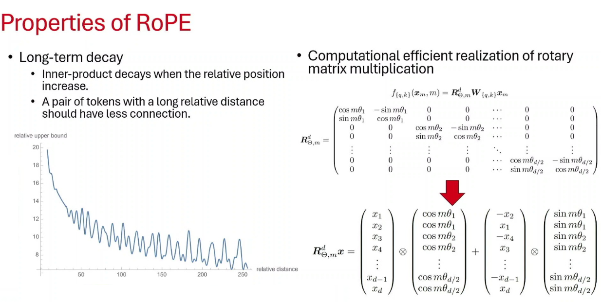
• Long-term decay: The graph on the left shows that as the relative distance between two tokens increases (x-axis), their positional dot product (y-axis) naturally decays. This is a highly desirable property, meaning the model naturally pays less attention to words that are very far away.

• Computational Efficiency: Multiplying a vector by that massive block-diagonal matrix would be incredibly slow. The bottom right of the slide shows a math trick. By segregating the cosine terms and sine terms, the complex matrix multiplication is simplified into basic element-wise multiplications and additions. This makes RoPE very fast to compute in hardware.

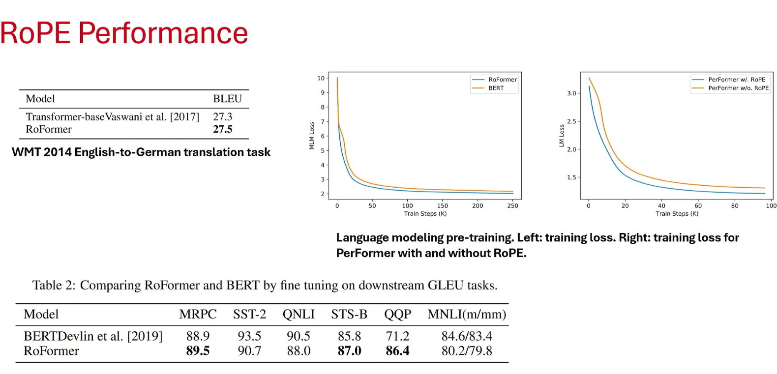(Results from the RoFormer paper (the model that introduced RoPE))

• Faster Convergence: The graphs show the training loss of RoFormer compared to BERT and Performer. The blue line (RoFormer) drops much faster than the orange line, indicating that RoPE helps the model learn the language faster and more efficiently.

• Better Accuracy: The tables show that simply swapping out the positional encoding method for RoPE yields noticeable improvements in BLEU scores (for translation) and GLUE benchmark tasks compared to the baseline models.

Summary

1. The Core Problem: The "Parallel" Blindspot

• Unlike older sequential models (RNNs), Transformers process all words simultaneously.

• Because the self-attention mechanism ($Q K^T$) is just a series of dot products, it is naturally blind to sequence order. Without explicit help, the model cannot distinguish "Dog bites man" from "Man bites dog."

• Naive attempts to fix this : like counting (1, 2, 3) or normalizing counts (0.1, 0.2, 0.3), fail mathematically because sequence lengths vary wildly, leading to unbounded growth or inconsistent vectors.

2. The Original Solution: Absolute Positional Encoding (Vaswani)

To solve the counting problem, the 2017 Transformer paper introduced a method of adding a unique pattern of continuous waves to the word embeddings before processing begins.

• The Blueprint: It creates a continuous, predictable vector of the exact same size as the word embedding ($d_{model}$) using alternating sine and cosine functions.

• High-Frequency Waves (The "Fast" Dimensions): The first few dimensions of the vector cycle up and down very rapidly. This creates a "sheer cliff" between adjacent words, ensuring the model never suffers from order blur (mixing up words that are right next to each other).

• Low-Frequency Waves (The "Slow" Dimensions): The later dimensions are stretched out massively by an exponentially growing denominator ($10000^{2i / d_{model}}$). These slow waves act as a long-range tape measure, allowing the model to uniquely identify a word's macro-position within a long paragraph without repeating.

• The Flaw: This is an Absolute encoding method. It assigns strict "seat numbers" to words. Because language is fluid, a network has to work extremely hard to figure out that shifting a whole sentence to the right doesn't actually change the relationship between the words in it.

3. The Paradigm Shift: Relative Distances

Researchers quickly realized that humans don't care about absolute seat numbers; we care about relative distances (e.g., "Word B is 3 steps away from Word A").

• Translation Invariance: If you shift a sentence, absolute seat numbers break, but relative distances remain perfectly intact.

• Models like Transformer-XL, DeBERTa, and T5 introduced mathematical hacks to the self-attention equation. They ripped out the absolute position vectors and explicitly forced the model to calculate attention based purely on the number of hops between the Query and the Key.

4. The Modern Standard: Rotary Positional Encoding (RoPE)

RoPE (used by LLaMA, PaLM, and most modern architectures) solved the absolute vs. relative debate by mapping word embeddings into the 2D complex plane and using rotation.

• Multiplicative, Not Additive: Instead of messing up the word's "meaning" vector by adding a position vector to it, RoPE leaves the magnitude alone and simply rotates the vector like the hands of a clock.

• The Complex Math Trick: By rotating the Query vector forward by its absolute position ($m$), and the Key vector forward by its absolute position ($n$), a mathematical phenomenon occurs during the dot product. Because the dot product requires a complex conjugate, the absolute positions natively subtract themselves ($m - n$).

• The Result: The model explicitly calculates absolute positions, but the self-attention mechanism only ever "sees" the relative angle (distance) between them. It is highly computationally efficient, features long-term decay (distant words naturally receive less attention), and drastically speeds up model training.