Transformers: Attention Is All You Need

Prerequisites :

• Attention 101
• Intution behind masked and cross attention
• Positional Encoding 101

Death of the RNN and the Parallelization Breakthrough

To appreciate why the Transformer architecture completely took over deep learning, we first have to understand the fundamental bottleneck it solved. Before 2017, if you wanted to build a sequence-to-sequence model for language translation or text generation, Recurrent Neural Networks (RNNs) and LSTMs were the undisputed state-of-the-art.

But RNNs had a fatal architectural flaw: they were strictly sequential. To understand a sentence, an RNN has to read it from left to right, one word at a time. Mathematically, it generates a hidden state $h_t$ as a function of the previous hidden state $h_{t-1}$ and the current word. You cannot process word number 50 until you have finished processing word number 49 which completely precludes parallelization. As sequence lengths grew longer, this sequential process created massive memory constraints and bottlenecked training times.

We started using CNNs for long text sequences which proved difficult. To connect two distant words using convolutions, you have to stack multiple layers, which means the number of operations required to relate distant words grows linearly or logarithmically depending on the architecture. This makes learning long-range dependencies incredibly difficult.

The Transformer's Solution: Drop the sequence, look at everything at once. Instead of processing a sentence word-by-word, it feeds the entire sequence into the model simultaneously. By relying entirely on the self-attention mechanism, the Transformer connects all positions in the input with a constant number of operations ($O(1)$), rather than the $O(n)$ sequential operations required by an RNN. Because every word's attention score can be calculated independently and simultaneously, the architecture finally allowed for massive parallelization across GPUs.

Solving Long Range Dependency Issues

Language is rarely confined to adjacent words. Often, the grammatical tense of a sentence or the identity of a pronoun is dictated by a word that appeared dozens or even hundreds of tokens earlier. In deep learning, this is known as the "long-range dependency" problem.

To understand why older models struggled with this, we have to look at how information physically travels through a neural network during training.

The ability of a model to learn these long-range connections is heavily affected by the length of the paths that forward and backward signals have to traverse within the network. The rule of thumb is simple: the shorter the path between any combination of positions in the input and output sequences, the easier it is to learn those long-range dependencies.

The Distance Bottleneck in RNNs and CNNs

In a Recurrent Neural Network (RNN), words are processed strictly in order. If you want the 50th word in a sentence to interact with the 1st word, the signal has to pass through 49 intermediate hidden states. Mathematically, the maximum path length between any two positions in an RNN is $O(n)$, where $n$ is the sequence length. Because the path is so long, the signal often dilutes or gets lost entirely (vanishing gradient problem). They tried CNNs for this. While CNNs allowed for parallel computation, they introduced a different problem. A single convolutional layer only looks at a small window of adjacent words (its kernel width) and does not connect all pairs of input and output positions. To make a word at the beginning of a sentence talk to a word at the end, you have to stack layers on top of each other like a pyramid. This increases the maximum path length to $O(n/k)$ (for contiguous kernels) or $O(\log_k(n))$ (for dilated convolutions), making it much more difficult to learn dependencies between distant positions.

The $O(1)$ Magic of Self-Attention

The Transformer solves this problem by completely flattening the distance between words. Instead of relying on sequential chains or stacked pyramids, the Transformer uses self-attention. In a self-attention layer, every single word in the sequence calculates a direct dot-product with every other word simultaneously. Because of this mechanism, a self-attention layer connects all positions with a constant number of sequentially executed operations. The maximum path length between any two words in the network, regardless of whether they are right next to each other or a thousand words apart, is strictly $O(1)$. By reducing the distance between all words to a single mathematical step, the Transformer guarantees that signals never degrade over long distances. It allows the model to instantly grasp context and seamlessly resolve long-range dependencies in a way previous architectures simply could not replicate.

Internals of a Transformer

So transformers comprise of two components i.e 'encoder' and 'decoder'.

• The Encoder (The Reader): Its entire job is to process the input text all at once and build a massive, mathematically rich understanding of what every word means in context.

• The Decoder (The Writer): Its job is to take that understanding and generate a response autoregressively, meaning it predicts the output one step at a time, using a "mask" to ensure it can't cheat by looking ahead at words it hasn't generated yet.

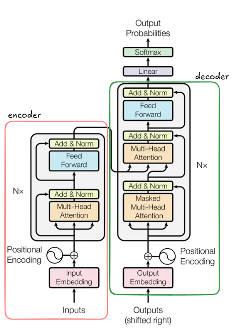
Neural networks cannot read English; they can only process numbers. Before a word even reaches the core Transformer engine, it has to be mathematically translated.

• Input Embeddings: First, words are mapped to unique IDs and projected into a dense multidimensional space. Think of this as a lookup table where each word gets assigned a vector of, for example, 512 numbers. These numbers act as coordinates. During training, the model constantly adjusts these numbers, moving words with similar meanings closer together in this 512-dimensional space.

• Positional Encoding: Because Transformers process all words in a sentence simultaneously rather than sequentially, they inherently have no concept of word order. To fix this, we inject a mathematical "time signature" into the embeddings. By adding a fixed vector calculated using interleaved sine and cosine functions, we give every position in the sentence a unique, relative identifier. This ensures the model knows the difference between "The dog chased the cat" and "The cat chased the dog."

The attention mechanism is what allows the model to look at a single word and determine how strongly it relates to every other word in the sequence.

• Queries, Keys, and Values: The model uses a database retrieval analogy. When analyzing a word, it acts as a Query (what the word is looking for), a Key (what the word is), and a Value (the core meaning of the word). The model calculates the dot product between the Query of one word and the Keys of all other words. A high score means a strong relationship, which mathematically amplifies that word's Value.

• The Projection Matrices: We don't just use the raw embeddings for this. The model learns specific weight matrices ($W^Q$, $W^K$, and $W^V$) that act like translation lenses. They rotate the base dictionary definition of a word into specific "Query" and "Key" spaces so verbs can efficiently search for nouns, and adjectives can search for subjects.

• Multi-Head Attention: If we calculated attention across all 512 dimensions at once, conflicting signals (like a strong grammatical match but an opposite emotional sentiment) would mathematically cancel each other out. To solve this "washing out" problem, the 512 dimensions are sliced into smaller chunks, or "heads." Each head operates independently, allowing the model to simultaneously evaluate grammar, emotion, and temporal context in parallel before concatenating the findings back together.

Processing thousands of matrix multiplications can cause numerical values to spiral out of control, making the model impossible to train. The architecture uses two tricks to keep the math stable :

• Layer Normalization: This forces the numbers inside a word's vector back into a healthy, consistent range (a mean of 0 and a variance of 1). Crucially, the model also learns two parameters ($\gamma$ and $\beta$) that allow it to stretch or shift these normalized values if it realizes a specific layer mathematically requires a wider variance.

• Residual Connections: These act as mathematical "bypass lanes." The original input to an attention block is added directly to its output. This prevents information loss and ensures gradients can flow smoothly backward during training without vanishing.

After the attention mechanism figures out how all the words relate to one another, the data passes into a fully connected Feed-Forward Network (FFN). If the attention layer is about words gathering context from their neighbors, the FFN is where each word individually processes that new context. It applies non-linear activation functions (like ReLU) to solidify complex patterns and decide what information is most important to pass to the next layer.

Once the data has cleared all the Encoder and Decoder blocks, the model has to turn its internal 512-dimensional understanding back into human language.

• Linear Projection: The final output vector is stretched out into an enormous array that matches the size of the model's entire vocabulary.

• Softmax Function: This mathematical function takes those raw, stretched-out numbers and converts them into a clean probability distribution. It forces all the values to sum to exactly 100%, allowing the model to make its final prediction by selecting the word with the highest probability.

So basically that was a brief view of internals of transformers, lets cover them one by one in depth.

Embeddings and Positional Encoding

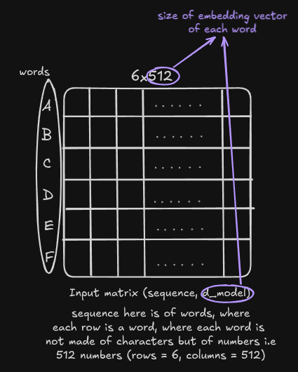(This is how the input looks like)

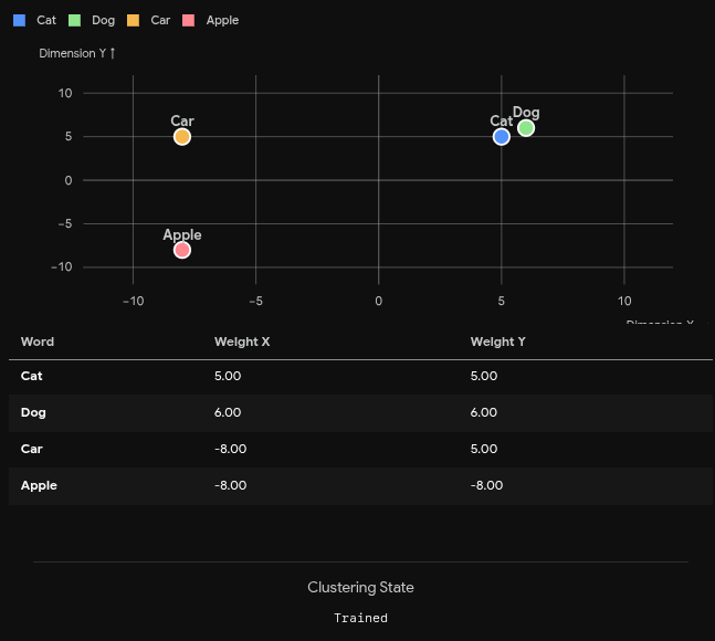
So we already know what embeddings are, they are continuous, dense vector representations of discrete tokens.

But how are these embeddings generated ?

Before training begins, the entire Embedding Matrix (every word has a row of 512 numbers) is filled with completely random numbers. At this stage, the model knows absolutely nothing. The vector for "CAT" is just as mathematically close to the vector for "APPLE" as it is to "DOG".

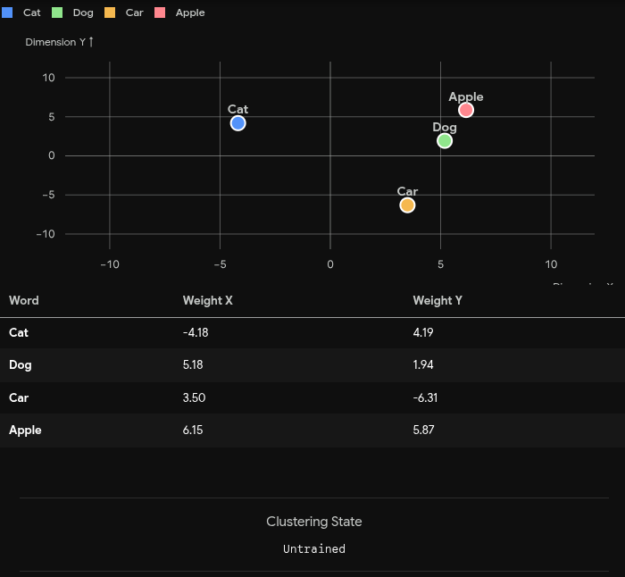
Then the forward pass takes place where the model is given a massive amount of text data and a task : usually predicting the next word in a sentence.

The system looks at the actual next word in the training data (which was "DOG"). It uses a mathematical function called a "Loss Function" to calculate exactly how wrong the model's guess was.

Then using backpropagation & gradient descent takes place where the model works backward from the error to figure out who is to blame. It calculates how every single number in the network, including the 512 numbers in the embedding vectors for the input words which contributed to the bad guess. This process is repeated billions of times across terabytes of text. Eventually, the multidimensional space organizes itself logically based strictly on how words are used together in language.

Embedding Pipeline :

Key steps in the pipeline are :

• Tokenization to Input IDs: The raw sequence is split into tokens, and each token is assigned a unique integer (e.g., "CAT" maps to 6587) based on its fixed position in the vocabulary.

• Vector Projection: These input IDs act as indices for a lookup table, mapping the discrete integer to a dense vector of a specific hidden dimension (often referred to as d_model). This projection creates a 512-dimensional vector.

• Learnable Parameters: While the vocabulary and input IDs are strictly fixed, the values within each embedding vector are not . These 512 numbers function as learnable weights. During backpropagation, the model dynamically updates these numerical values to minimize the loss function.

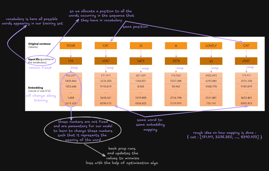
By continuously adjusting these weights during training, the model shapes the multidimensional space so that vectors representing semantically related tokens are positioned closer together.

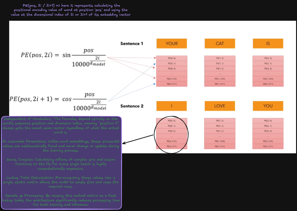
Encoding Pipeline :

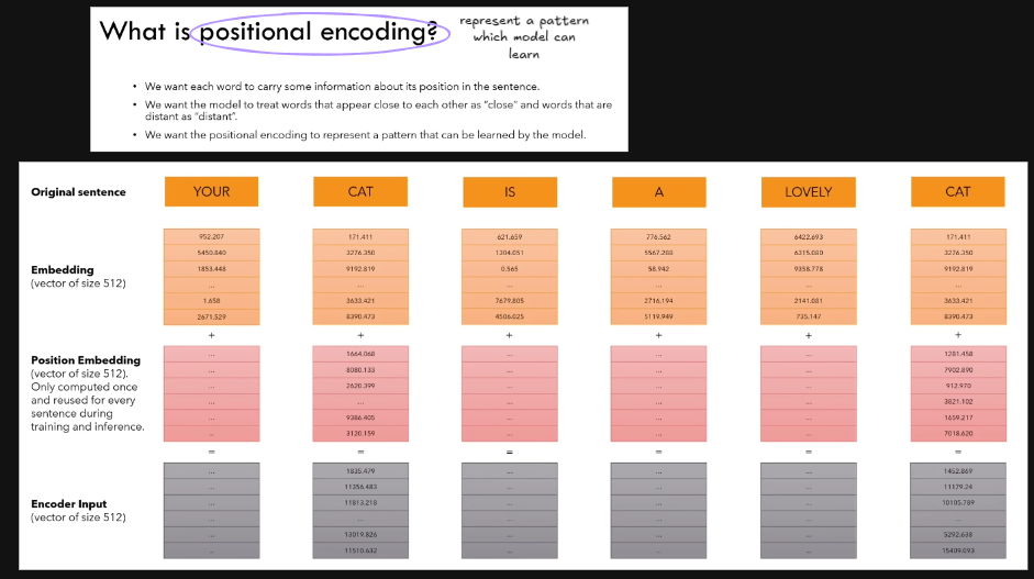
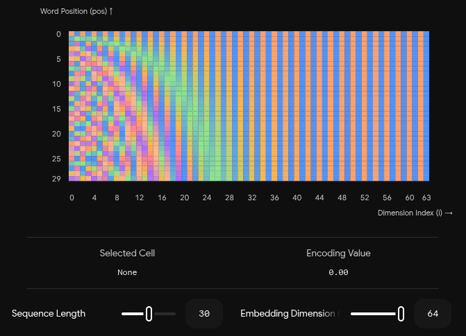
Why did we pair sine and cosine like this ?

The choice to interleave these specific trigonometric functions is for two main reasons :

1. Representing Relative Distance: By pairing a sine and cosine function at the same frequency, the model can easily calculate the relative distance between any two words. Mathematically, for any fixed offset $k$ (e.g., a word that is exactly 3 positions away), the positional encoding at $pos + k$ can be represented as a linear transformation of the positional encoding at $pos$. This makes it incredibly easy for the attention mechanism to learn patterns like "pay attention to the word exactly two spots before this one."

2. The "Clock" Analogy: The denominator in those equations ($10000^{2i/d_{model}}$) scales based on the dimension index $i$. This means the early dimensions (like index 0 and 1) have a very high frequency, they change rapidly from word to word. As you go deeper into the vector (e.g., dimension 500 and 501), the frequency becomes extremely low, barely changing across a short sentence. It functions like the hands on a clock: the seconds hand spins fast, the minute hand moves slower, and the hour hand moves the slowest. This combined state provides a completely unique "time signature" for every absolute position.

Why do we calculate positional encoding once then re-use it ?

The reason we calculate positional encodings only once and reuse them boils down to two key factors : mathematical independence and computational efficiency.

1. The Math is Completely Independent of the Words

If you look closely at the formulas for positional encoding, the output depends on exactly two variables :

• pos: The index of the word in the sentence (0, 1, 2...).
• i: The dimension index inside the vector (0 to 511).

Notice what is missing: the actual word itself. The formula does not care if the word at position 0 is "YOUR", "I", "APPLE", or "THE". The mathematical output for position 0 will always be the exact same vector of 512 numbers. Because the result is deterministic and strictly tied to the slot rather than the content, there is no need to recalculate it for different sentences.

2. There are No Learnable Parameters

Unlike word embeddings, which start as random numbers and are constantly updated during training via gradient descent, these specific sinusoidal positional encodings are entirely fixed. The model never adjusts the sine and cosine values. Because they never change during training, recalculating them at every step would be completely redundant.

(Note: Some newer models do use "learned" positional embeddings that change during training, but the original Transformer paper discussed in the video uses this fixed mathematical approach).

3. Saving Compute (The "Lookup Table" Optimization)

Calculating sine and cosine functions for millions of data points is computationally expensive for a CPU or GPU. Instead of doing this math on the fly for every single word in every single batch of text, developers use a caching strategy:

1. When the model is initialized, the computer calculates a massive matrix of these positional encodings up to the model's maximum sequence length (e.g., up to position 2048).
2. It saves this matrix in memory.
3. During training or inference, when a sentence of length $N$ comes in, the model simply slices the first $N$ rows from this pre-calculated matrix and adds them to the word embeddings.

Attention

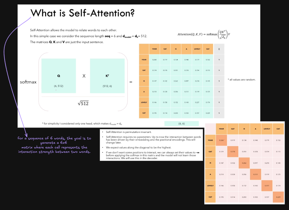
So let's breakdown how the attention process takes place in transformers :

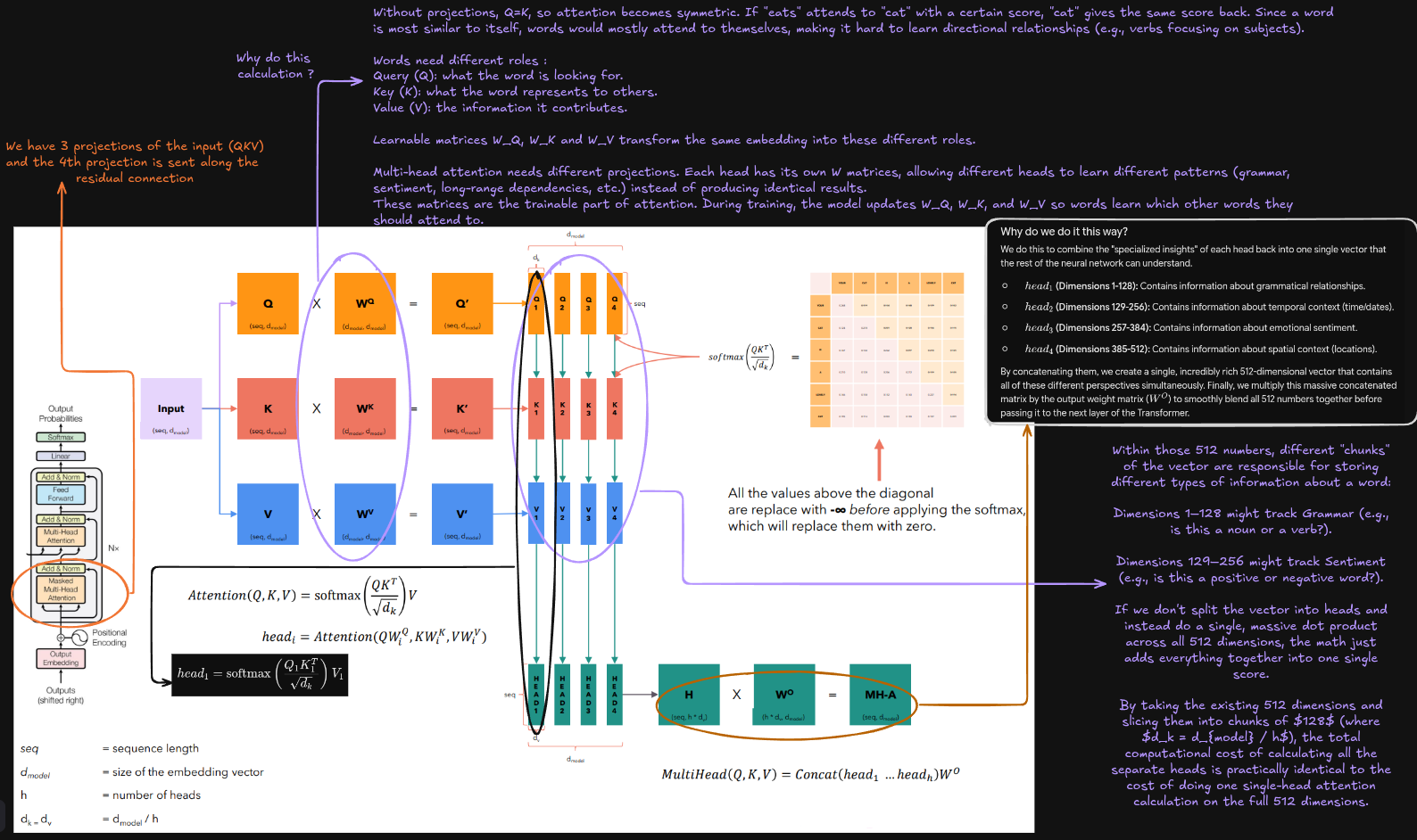(Right Click on the image -> Open in new tab, to read clearly)

• The input sequence makes three copies of itself to serve as Queries ($Q$), Keys ($K$), and Values ($V$), and 4th copy is sent along residual connection
• These 3 projections are multiplied by three separate, learnable parameter matrices: $W^Q$, $W^K$, and $W^V$.
• This transformation creates the projected matrices $Q'$, $K'$, and $V'$.

But why multiply those 3 projections with $W^Q$, $W^K ~and$ $W^V$ ?

If we didn't have the $W^Q$, $W^K$, and $W^V$ projection matrices, we would just be calculating the attention using the raw input embeddings directly. That would cause three massive mathematical problems :

1. Words would only pay attention to themselves (Symmetry)

Imagine the sentence: "The cat eats." If we use the raw embeddings without projecting them, then $Q = K$.

When the word "eats" calculates its attention score with "cat", it does a dot product: $Embedding_{eats} \cdot Embedding_{cat}$.

When "cat" calculates its attention score with "eats", it does the exact same math: $Embedding_{cat} \cdot Embedding_{eats}$.

Because the dot product is symmetric, "eats" would pay the exact same amount of attention to "cat" as "cat" pays to "eats." Worse, a vector's dot product with itself is always its maximum value. Every word would just look mostly at itself, and we would never learn complex, one-way relationships like "a verb focuses on its subject."

2. A word needs different "Roles"

A single word in a sentence is doing three different jobs simultaneously. Let's look at the word "eats":

• As a Query (Q): It is asking the sentence, "I am an action. Where is the noun that is performing me?"
• As a Key (K): It is telling the sentence, "I am a singular verb representing consumption."
• As a Value (V): It is providing its core semantic meaning to the final output.

"What I am looking for" (Query) is fundamentally different from "What I am" (Key). The learnable weights ($W^Q$, $W^K$, $W^V$) act as translation lenses. They take the base dictionary definition of the word and mathematically rotate/stretch it into a specific "Query space," a "Key space," and a "Value space" so these distinct roles can interact.

3. There would be no "Multi" in Multi-Head Attention

If we didn't use projection matrices to split the inputs, every single attention head would just be taking the exact same raw embedding, doing the exact same dot product, and getting the exact same result. It would be entirely redundant.

By having different, independent $W$ matrices for each head (e.g., $W^Q_1$, $W^Q_2$, $W^Q_3$), the model learns to project the exact same word into totally different conceptual spaces. Head 1's matrices might project the words into a space that analyzes grammar (verbs finding nouns). Head 2's matrices might project them into a space that analyzes sentiment (positive words finding negative words).

The $W$ matrices are the actual parameters that get updated during backpropagation. When a Transformer is "training," what it is actually doing is tweaking the numbers inside $W^Q$, $W^K$, and $W^V$ so that words project into vectors that perfectly align with the words they are supposed to pay attention to.

Why we split ($Q'$, $K'$, $V'$) into separate chunks (heads) ?

1. The "Washing Out" Problem (Representation Subspaces)

Imagine we have a single embedding vector with 512 dimensions. Within those 512 numbers, different "chunks" of the vector are responsible for storing different types of information about a word :

• Dimensions 1–128 might track Grammar (e.g., is this a noun or a verb?).
• Dimensions 129–256 might track Sentiment (e.g., is this a positive or negative word?).

If we don't split the vector into heads and instead do a single, massive dot product across all 512 dimensions, the math just adds everything together into one single score.

If word A and word B are a perfect grammatical match (generating a huge positive number) but have exact opposite sentiments (generating a huge negative number), those two numbers will cancel each other out during the dot product. The final attention score will be zero. The model completely misses the grammatical connection because the sentiment difference "washed it out."

By splitting the 512-dimensional matrix into 4 separate heads of 128 dimensions:

• Head 1 calculates attention only on the grammar dimensions. It finds a strong connection!
• Head 2 calculates attention only on the sentiment dimensions. It finds no connection.

When we concatenate them back together at the end, the model preserves both pieces of information: "These words are grammatically linked, but emotionally opposite." Splitting allows the model to attend to information from different "subspaces" simultaneously without them interfering with one another.

2. Computational Efficiency

If you look closely at the math, splitting the matrices is an elegant optimization trick. If we wanted to give the model 4 different perspectives (4 heads) but kept the full 512 dimensions for every single head, the computational cost would be $4 \times$ higher. By taking the existing 512 dimensions and slicing them into chunks of $128$ (where $d_k = d_{model} / h$), the total computational cost of calculating all the separate heads is practically identical to the cost of doing one single-head attention calculation on the full 512 dimensions. You get the benefit of multiple specialized perspectives without increasing the math burden on the GPU.

After the split heads do their specialized jobs, we have a bunch of small 128-dimensional output vectors. The rest of the Transformer architecture (like the Feed Forward layers) is strictly designed to process 512-dimensional vectors. Concatenating the small chunks side-by-side perfectly reconstructs a 512-dimensional vector. That final multiplication by $W^O$ (the output matrix) acts as a blender, it smoothly mixes the distinct insights from all the separate heads together into a final, unified representation that the next layer can easily read.

We have four separate output matrices: $head_1$, $head_2$, $head_3$, and $head_4$. Because our original embedding size ($d_{model}$) was 512, and we split it into 4 heads, each of these output matrices is exactly 128 dimensions wide.

This is where the concatenation happens. We glue the outputs of the heads together side-by-side : $128 + 128 + 128 + 128 = 512$

By concatenating $head_1$, $head_2$, $head_3$, and $head_4$, we perfectly rebuild a full 512-dimensional matrix. We do this to combine the "specialized insights" of each head back into one single vector that the rest of the neural network can understand.

• $head_1$ (Dimensions 1-128): Contains information about grammatical relationships.
• $head_2$ (Dimensions 129-256): Contains information about temporal context (time/dates).
• $head_3$ (Dimensions 257-384): Contains information about emotional sentiment.
• $head_4$ (Dimensions 385-512): Contains information about spatial context (locations).

By concatenating them, we create a single, incredibly rich 512-dimensional vector that contains all of these different perspectives simultaneously. Finally, we multiply this massive concatenated matrix by the output weight matrix ($W^O$) to smoothly blend all 512 numbers together before passing it to the next layer of the Transformer.

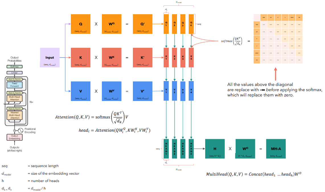(Un-annotated version of the attention process)

Layer Normalization

In the Transformer architecture, as data passes through various layers (like Multi-Head Attention and Feed-Forward networks), the numerical values can grow wildly large or shrink drastically. If these numbers become too extreme, it causes the "vanishing/exploding gradient" problem, making the model unstable and nearly impossible to train.

Layer Normalization is the mechanism used to forcefully stabilize these values, keeping them in a healthy, consistent range.

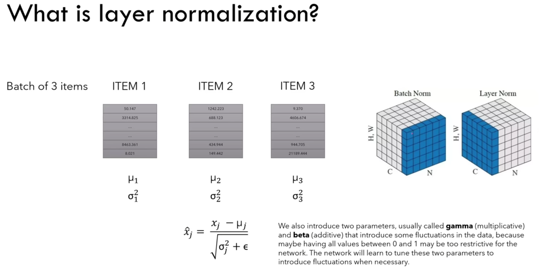
1. The Core Calculation (Per Item)

In a Transformer, an "item" is a single word token represented by its 512-dimensional embedding vector. Instead of looking at the entire sentence at once, Layer Normalization isolates a single word (e.g., "ITEM 1"). It looks at the 512 numbers inside that specific word's vector and calculates:

• The Mean ($\mu$): The average of those 512 numbers.
• The Variance ($\sigma^2$): How spread out those 512 numbers are from the mean.

It then applies the standard normalization formula shown at the bottom : $\hat{x}_j = \frac{x_j - \mu_j}{\sqrt{\sigma_j^2 + \epsilon}}$ (Note: The $\epsilon$ is just a tiny number like 0.00001 added to prevent accidentally dividing by zero). This formula transforms the vector so that its new mean is exactly 0 and its variance is exactly 1. It centers the data.

2. Batch Norm vs. Layer Norm (The Cubes)

The 3D cubes on the right highlight why Transformers use Layer Norm instead of the older Batch Norm (which is common in CNNs).

• Batch Norm (Left Cube): Calculates the mean and variance across the entire batch of sentences for a single feature. This is terrible for NLP because sentences are all different lengths (lots of padding tokens), which completely throws off the batch-wide statistics.

• Layer Norm (Right Cube): Calculates the mean and variance across all features (the 512 dimensions) for a single word. It completely ignores the rest of the batch and even the other words in the sentence. This makes it perfectly stable regardless of how long the sentence is.

3. Gamma ($\gamma$) and Beta ($\beta$) - The "Un-normalizers"

You might notice a problem : if we force every single word vector to have a mean of 0 and a variance of 1, we might accidentally destroy the unique mathematical variations that the attention mechanism just worked so hard to learn.

To fix this, the network introduces two new learnable parameters:

• Gamma ($\gamma$): A multiplier that scales the data (stretches or shrinks the variance).
• Beta ($\beta$): An additive term that shifts the data (moves the mean up or down).

After applying the strict normalization formula, the model calculates:

$\text{Output} = \gamma \hat{x}_j + \beta$

Why do this? It gives the neural network the choice. If strict normalization is helpful, it will learn to set $\gamma = 1$ and $\beta = 0$. But if the network realizes that a specific layer actually needs a larger variance or a shifted mean to capture complex language patterns, backpropagation will adjust $\gamma$ and $\beta$ to stretch and shift the data exactly where it needs to be. It provides stability without sacrificing flexibility.

Training

Before Transformers, models like Recurrent Neural Networks (RNNs) had to be trained sequentially. To translate a 10-word sentence, the model had to run 10 separate times, waiting for the previous word to be generated before it could guess the next one.

In a Transformer, it all happens in one time step. This is how the pipeline works :

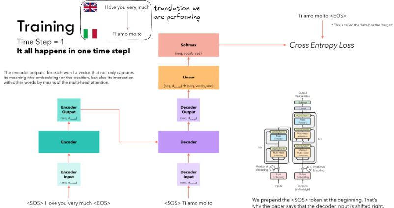
1. The Setup (Two Inputs at Once)

During training, we already know the answer. We have the English sentence and the perfect Italian translation. Instead of making the model guess blindly from the start, we feed data into both sides of the network simultaneously i.e Teacher Forcing :

• Encoder Input: The complete source sentence, wrapped in special tokens: <SOS> I love you very much <EOS>. The encoder processes this and outputs its rich, context-heavy matrices (Keys and Values).

• Decoder Input ("Shifted Right"): We take the target Italian sentence, put a Start-of-Sentence token at the front, and chop off the End-of-Sentence token: <SOS> Ti amo molto.

2. The "Cheat" Prevention (Causal Masking)

Because we feed the entire Italian sentence into the decoder all at once, the model mathematically has access to the "answers." If it is trying to predict the word following "Ti", it could just look at the next input token ("amo") and copy it.

This is exactly why the Masked Multi-Head Attention (which we discussed earlier) is placed at the very bottom of the decoder. The $-\infty$ mask blinds the model to future words.

• At position 1 (<SOS>), the mask only lets it see <SOS>.
• At position 2 (Ti), the mask lets it see <SOS> and Ti.
• It is forced to learn the patterns of language without peeking at the rest of the matrix.

3. The Predictions (Linear & Softmax)

The decoder outputs a matrix representing its predictions for the sequence.

• The Linear layer takes these 512-dimensional output vectors and stretches them out to the size of your entire vocabulary (e.g., 50,000 words).

• The Softmax layer turns those 50,000 raw numbers into a probability distribution. For each position in the sentence, the model generates a percentage guess for what the next word should be out of all 50,000 possible words.

4. The Grader (Cross Entropy Loss)

Now, the model's simultaneous guesses are compared against the actual target Label: Ti amo molto <EOS>. Notice how the target label aligns with the decoder's input :

• Input: <SOS> $\rightarrow$ Target expected: Ti
• Input: Ti $\rightarrow$ Target expected: amo
• Input: amo $\rightarrow$ Target expected: molto
• Input: molto $\rightarrow$ Target expected: <EOS>

The Cross Entropy Loss calculates exactly how mathematically far off the model's probability distribution was from the correct 100% target. Because this is calculated for the entire sequence simultaneously in a single massive matrix multiplication, the system backpropagates the loss and updates the weights for every single word at the exact same time.

Researchers utilized the Adam optimizer and customized how the learning rate behaved over time. If a model starts training with a massive learning rate while its weights are still completely random, it can destabilize immediately. Conversely, if the learning rate is too small, the model will take an eternity to learn. To solve this they implemented a specific learning rate schedule. They set the model to undergo a "warmup" phase for the first 4,000 training steps. During this warmup window, the learning rate increased linearly, allowing the model to quickly safely accelerate its learning process. Once those 4,000 steps were completed, the learning rate didn't just stay flat. It was programmed to gradually decrease proportionally to the inverse square root of the step number. This meant that as the model got closer and closer to its optimal state, it took smaller, more careful mathematical steps, allowing it to fine-tune its translation accuracy without overshooting the target.

The researchers trained their base models on a single machine equipped with eight NVIDIA P100 GPUs. The base model required only 100,000 steps to train, which took a mere 12 hours. Transformer's self-attention mechanism allowed for unprecedented parallelization, the hardware requirements plummeted. Their massive Transformer (big)" model only required 3.5 days of training. This larger model went on to establish a brand new single-model state-of-the-art BLEU score of 41.0 on the WMT 2014 English-to-French translation task.

Inference

Unlike the training phase, where the model processes the entire output sequence simultaneously, Inference (generating text in the real world) is strictly an autoregressive, step-by-step loop. Because the model doesn't know the future, it has to generate one word, append it to its own input, and run again.

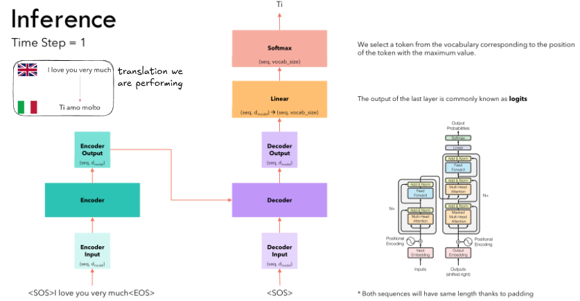
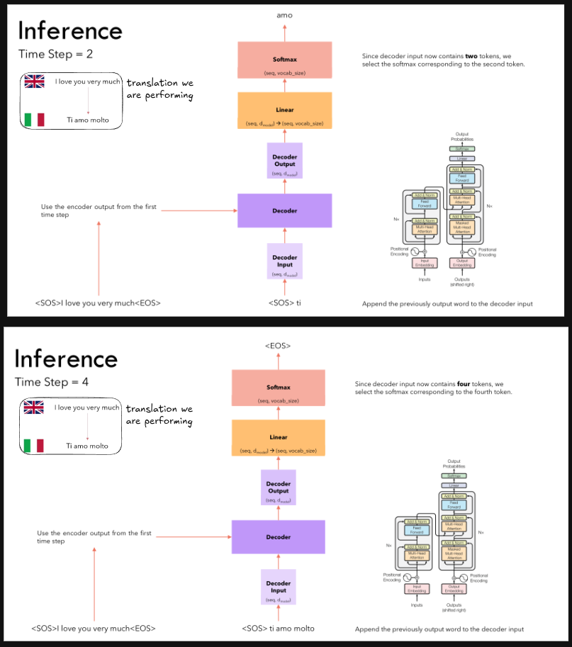
This is how the inference pipeline works (the autoregressive loop (time steps 1-4)) :

1. The Static Encoder (Happens Once):

   Before any text is generated, the full input sentence ("<SOS> I love you very much <EOS>") is passed through the Encoder. The Encoder produces a rich set of Keys ($K$) and Values ($V$). Because the English sentence never changes, the model caches this output. It does not need to be recalculated for the rest of the generation process.

2. Time Step 1 (The First Guess):

   • Input: The Decoder is fed only the <SOS> (Start of Sentence) token.
   • Cross-Attention: Inside the Decoder, the <SOS> token acts as the Query ($Q$), looking at the cached $K$ and $V$ matrices from the Encoder to understand the context of the English sentence.
   • Output: The model outputs a probability distribution over the entire vocabulary. It selects the word with the highest probability: "Ti".

3. Time Step 2 (Appending the Output):

   • Input: The model takes its previous prediction ("Ti") and appends it to the input. The new input is now <SOS> Ti.
   • Output: The model processes this new sequence, queries the Encoder again, and predicts the next word: "amo".

4. Time Step 3 & 4 (The Loop Continues):

   • Time Step 3 Input: <SOS> Ti amo $\rightarrow$ Predicts "molto".
   • Time Step 4 Input: <SOS> Ti amo molto $\rightarrow$ Predicts <EOS>. Once the model predicts the <EOS> (End of Sentence) token, the inference loop officially terminates. The final translation is complete.

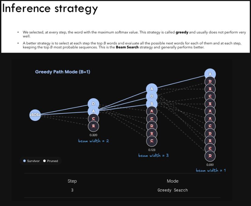
The model always picked the absolute most probable word at every single step. This is called Greedy Search.

• The Flaw of Greedy Search: Sometimes, picking the mathematically safest word right now forces the model into a grammatical corner later, resulting in a clunky or incorrect sentence overall.

• The Beam Search Solution: Instead of picking just one word, the model keeps the top $B$ possibilities alive (where $B$ is the "beam width").

  • If $B = 3$, at Time Step 1, the model saves the top 3 best words (e.g., "Ti", "Io", "Noi").

  • At Time Step 2, it explores the next possible word for all three of those paths, calculates the combined probability of the sequences, and prunes the list back down to the 3 best overall paths.

  • This allows the model to look slightly ahead and choose a path that might have a slightly lower initial probability but leads to a much better sentence structure overall.

Token Padding

To process text efficiently, neural networks rely on massive parallel computations performed by GPUs. GPUs are incredibly fast, but they are incredibly rigid: they only understand perfectly shaped rectangular matrices (tensors).

This introduces a physical problem. Human language is highly variable. If you feed a batch of three sentences into a model, they might look like this :

• Sentence 1: "I love cats" (3 words)
• Sentence 2: "Transformers are powerful" (3 words)
• Sentence 3: "The quick brown fox jumps over the lazy dog" (9 words)

You cannot stack a row of 3, a row of 3, and a row of 9 into a perfect rectangle. Padding is the engineering trick used to force these variable-length sequences into a uniform matrix shape so the GPU doesn't crash.

This is how the padding pipeline works :

1. Define the Sequence Length

First, the system determines the target length for the batch. This is usually either:

• Dynamic padding: The length of the longest sentence currently in the batch (in our example, 9 words).

• Fixed padding: A hardcoded maximum limit set by the model architecture (e.g., GPT-2's max length of 1024 tokens).

2. Add the <PAD> Tokens

For every sentence that is shorter than the target length, the model appends a special, meaningless dummy token, usually represented as <PAD> or an ID like 0, until the sentence reaches the exact required length.

• "I love cats" becomes "I love cats <PAD> <PAD> <PAD> <PAD> <PAD> <PAD>".

Now, every sentence in the batch is exactly 9 tokens long, creating a perfect $3 \times 9$ matrix that the GPU can process simultaneously.

3. The Attention Mask (Hiding the Dummy Data)

Padding solves the GPU geometry problem, but it introduces a mathematical problem. If the attention mechanism calculates interactions across the whole 9-token sequence, the word "cats" might accidentally start paying attention to the <PAD> tokens, which would corrupt the meaning of the sentence.

To prevent this, the tokenizer simultaneously generates an Attention Mask. This is a secondary matrix composed entirely of 1s and 0s.

• 1 means "This is a real word; pay attention to it."
• 0 means "This is a dummy <PAD> token; completely ignore it."

Before the softmax function is applied in the attention layer, the model multiplies the raw attention scores by this mask (or applies a $-\infty$ penalty), ensuring the <PAD> tokens mathematically disappear from the context calculations.

Opening the Black Box (Interpretability)

Deep learning models, especially dense neural networks, have long been plagued by the "black box" problem. You feed data in, you get predictions out, but figuring out why the model made a specific decision is notoriously difficult. The inner workings are usually a tangled mess of millions of floating-point numbers that mean nothing to a human observer.

The Transformer, however, brought a new level of transparency to NLP. Because self-attention explicitly assigns a mathematical weight to every single word-to-word interaction, it inherently acts as a window into the model's reasoning.

The authors of the Attention Is All You Need paper noted this as a highly valuable side benefit : self-attention architectures naturally yield much more interpretable models. By mapping the attention scores into visual distributions (like the connection lines we often see in Transformer diagrams), researchers could literally watch the model "think" and analyze exactly which words it was focusing on during translation. Researchers found the model was organically learning the underlying rules of human language.

First, they observed that the multi-head architecture was doing exactly what it was designed to do: individual attention heads clearly learned to perform completely different, specialized tasks. One head might focus exclusively on finding the subject of a sentence, while another head might focus entirely on resolving pronouns to their correct nouns.

More importantly, the researchers noted that many of these attention heads appeared to exhibit behavior directly related to the syntactic and semantic structure of the sentences. Without ever being explicitly programmed with a dictionary or a grammar rulebook, the Transformer was mapping out the linguistic structure of English purely through the geometry of its attention matrices.

This inherent interpretability didn't just make the model fascinating to study, it made it significantly easier for engineers to debug, trust, and eventually scale into the massive architectures we see today.

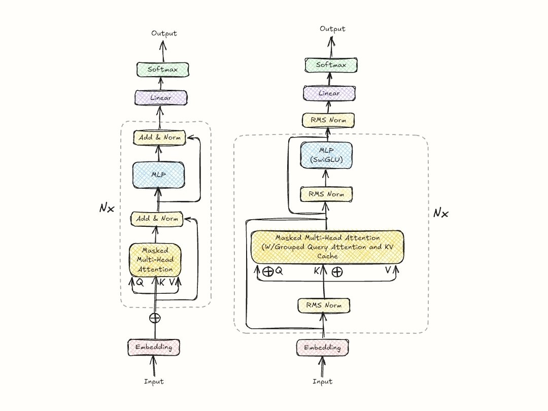
Paper Link : https://arxiv.org/pdf/1706.03762

You can find the code for this at :